Menu


As a digital marketer, you’ve got a lot on your plate. And you need tools that are versatile. Tools that you can use for more than one task. One of those tools is Google Sheets. Google Sheets is one of the most popular tools for digital marketing. It gives you a bunch of powerful features, is free, and is easy to collaborate with team members.
Digital Marketers use Google Sheets to store data, track KPIs, plan media campaigns, and more. And if you know how to use it effectively, it can streamline your workflow. In this article, you’ll learn the top 10 tips for using Google Sheets efficiently.
These time-saving shortcuts can help you speed up your workflow. Let’s look at 10 of the most useful.
Ctrl + / (PC and Mac)
F4 (PC and Mac)
Ctrl + R (PC)
Command + R (Mac)
Ctrl + D (PC)
Command + D (Mac)
Ctrl + Enter (PC)
Command + Enter (Mac)
Ctrl + Space
Shift + Space
Ctrl + \ (PC)
Command + \ (Mac)
Ctrl + ` (PC and Mac)
Shift + F11 (PC)
Shift + Fn + F11 (Mac)
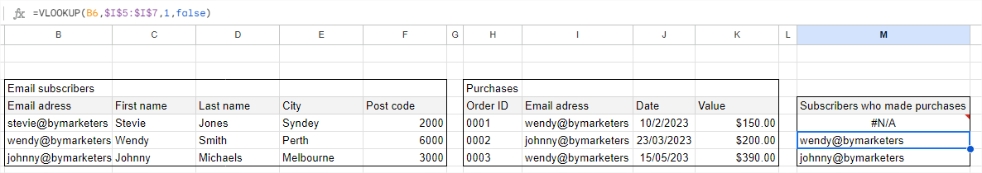
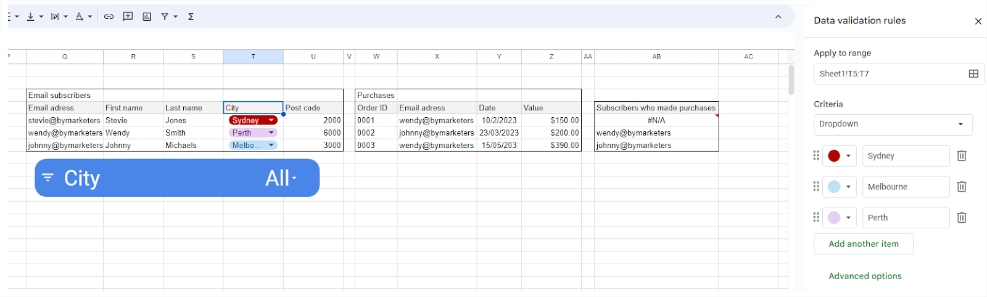
The VLOOKUP function in Google Sheets finds information across multiple sheets or ranges. It looks up matching data and then puts it in a different cell.
For example, let’s say you have a list of purchases and customer information in one sheet and a list of email subscribers in another. You can use VLOOKUP to find which subscribers have made purchases. And which haven’t — signaled by the #N/A return.
Here’s how the syntax looks:
| VLOOKUP (search_key, range, index, [is_sorted]) |
It’s not as confusing as it looks. The search key is the email address of the subscribers. The range is the email address of customers. The index is the number of the column that has the data you want. And false at the end shows the data isn’t sorted.
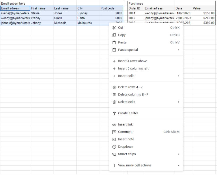
You can use filters to show only the most relevant data. To add a filter, select the range, right-click, and select Create a filter.
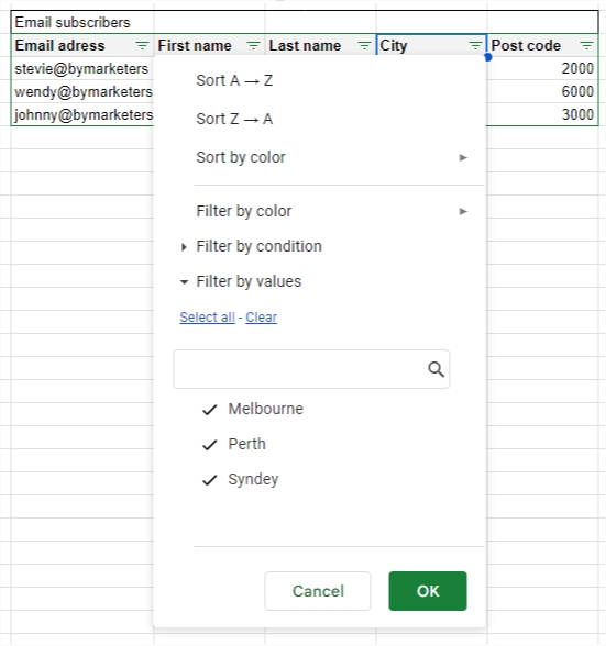
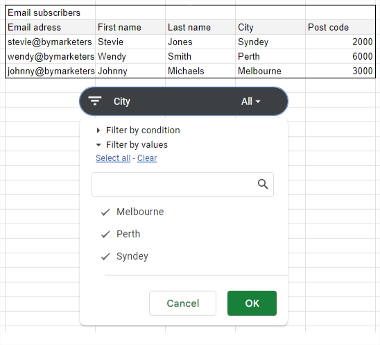
When you’ve done that, you’ll see a triangle in the top-row cells. Click the triangle and you can select what data you want to see. Let’s go back to our email subscribers example. You can use a filter to find your subscribers in a specific city so you can personalize your marketing content. You can also filter by condition, and sort your data from the filter menu.
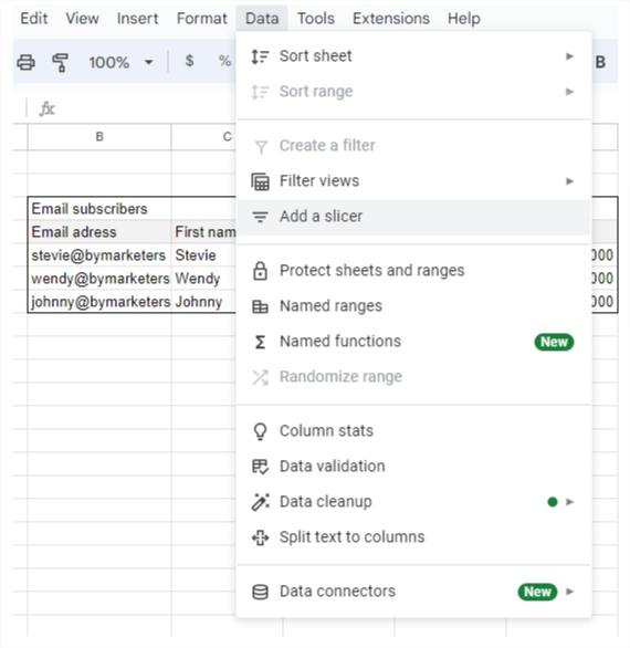
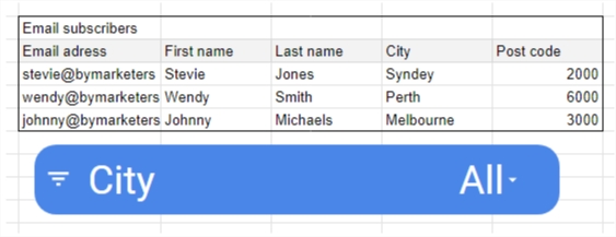
A slicer is similar to a filter — you can use it to select which data you want to see — but instead of showing a small triangle in a cell, you get an interactive toolbar. To add a slicer, choose Add a slicer from the Data menu. Follow the prompts and select a data range and column to filter by.
Next, choose the data you want to see from the Slicer toolbar.
One of the best reasons to use a Slicer over a Filter is the customization. You can change font, font size, background color, and toolbar size. This means you can make your sheets more like interactive dashboards than spreadsheets.
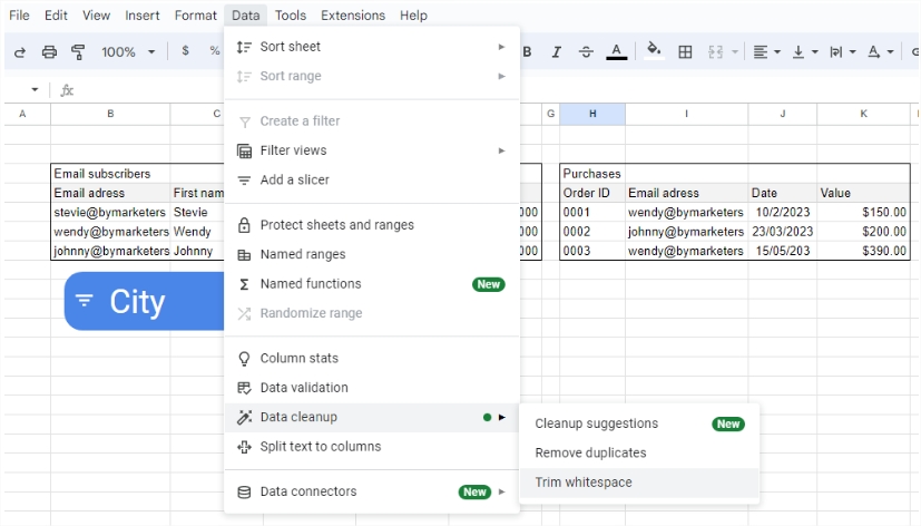
This one is a huge time saver. If you’ve ever spent time deleting duplicates from a dataset or getting rid of double spaces, you’ll know what I mean. From the Data menu, select Data cleanup and Google Sheets will do it for you.
To speed up data input, you can easily make dropdown lists. Select Data validation from the Data menu. Select the cell or range you want the dropdown list in. Choose Dropdown or Dropdown (from a range) from the Criteria list. If you select Dropdown, input the options. If you choose dropdown (from a range) select the list you want to appear. Now you don’t need to manually type the data — you can just click and select the value.
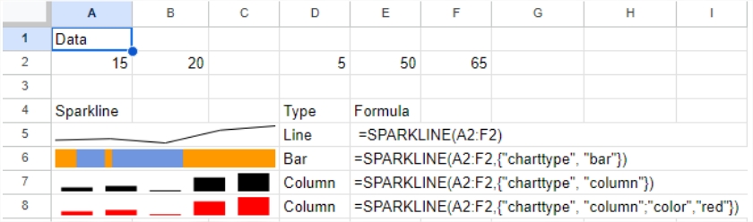
Sparklines are mini charts that you can include in a cell. They come in a bunch of types with customization options. For example, you can track your social media metrics over a period of time in a cell. This can be useful on a sheet packed full of data as you might not have enough space to input a large chart.
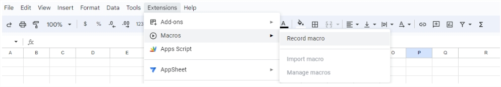
Macros are an advanced tool you can use to automate tasks you always have to repeat. These repetitive and boring tasks can take up a lot of your time. Think of those tasks you need to do in Google Sheets every day. They’re prime targets for automation.
To set one up, from the Extensions menu, select Macros and Record macro. Choose absolute or relative references and perform the task. Google Sheet records the task and you can name and save the macro. From now on, access the macro from the Tools menu and save yourself a bunch of time.
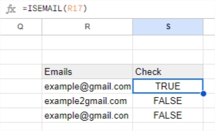
Digital marketers spend a lot of time collecting customer data and information. And one big challenge is making sure it’s accurate. One easy way to check if customers have inputted their email addresses correctly is the =ISEMAIL function. Just select the cell you want to check, and the function returns TRUE if it’s a valid email address. And FALSE if it isn’t.
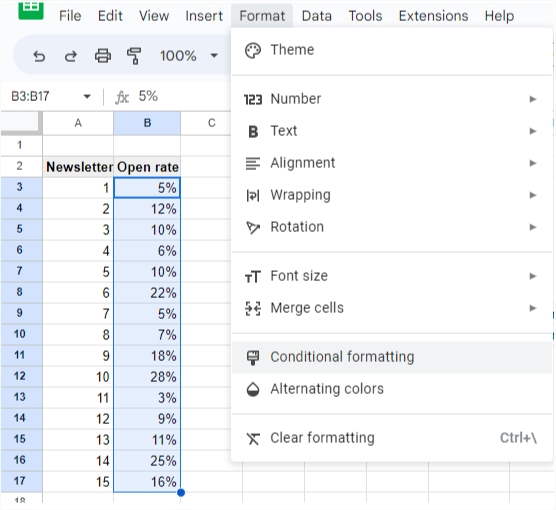
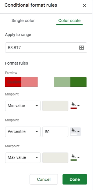
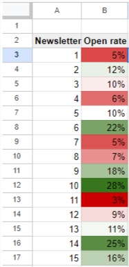
Heatmaps are a great way to add color to a data set. Take a look at this small dataset about email open rates. At a glance, it’s hard to see which newsletters did well and which didn’t. So let’s add color to make it clearer. From the Format menu choose Conditional Formatting.
Choose the Color scale format and decide your color scheme.
Now it’s much easier to see which newsletters engaged your audience and which didn’t.
Most shortcuts in excel are also available in Google Sheets. To enable Excel shortcuts in Google Sheets turn on “Enable compatible spreadsheet shortcuts” in the Keyboard shortcuts settings under the Help dropdown or by pressing Ctrl+/.
Google Sheets is a versatile platform that digital marketers can use in many ways. They can use it to analyze their website traffic, track their ecommerce performance, understand TikTok performance metrics, and more. Read more about the best Google Sheets templates for digital marketers.
In most aspects, yes. XLOOKUP is considered a more versatile function as it can look for values to both the left and right of the lookup array. VLOOKUP can only look to the right.
Digital marketers love Google Sheets because it’s easy to use. It doesn’t cost a penny. You can use it anywhere on any device. And you can easily share and customize your spreadsheets.
Of course. Check out the full range of Google Sheets resources on byMarketers. You’ll find everything from cash flow trackers and resources to help you create engaging newsletters to business planners.